Introduction
The hubEnsembles package provides a flexible framework
for aggregating model outputs, such as forecasts or projections, that
are submitted to a hub by multiple models and combined into ensemble
model outputs. The package includes two main functions:
simple_ensemble and linear_pool. We illustrate
these functions in this vignette, and briefly compare them.
This vignette uses the following R packages:
Example data: a forecast hub
We will use an example hub provided by the hubverse to demonstrate
the functionality of the hubEnsembles package. This example
hub was generated with modified forecasts from the FluSight forecasting
challenge, a collaborative modeling exercise run by the US Centers for
Disease Control and Prevention (CDC) since 2013 that solicits seasonal
influenza forecasts from outside modeling teams. The example hub
includes both example model output data and target data (sometimes known
as “truth” data), which are stored in the hubExamples
package as data objects named forecast_outputs and
forecast_target_ts. Note that the toy model outputs contain
predictions for only a small subset rows of select dates, locations, and
output type IDs, far fewer than an actual modeling hub would typically
collect.
The model output data includes quantile, mean and median forecasts of
future incident influenza hospitalizations and PMF forecasts of
hospitalization intensity (categories determined by threshold of weekly
hospital admissions per 100,000 population). Each forecast is made for
five task ID variables, including the location for which the forecast
was made (location), the date on which the forecast was
made (reference_date), the number of steps ahead
(horizon), the date of the forecast prediction (a
combination of the date the forecast was made and the forecast horizon,
target_end_date), and the forecast target
(target). Below we print a subset of this example model
output.
hubExamples::forecast_outputs |>
  dplyr::filter(
    output_type %in% c("quantile", "median", "pmf"),
    output_type_id %in% c(0.25, 0.75, NA, "low", "moderate", "high", "very high"),
    reference_date == "2022-12-17",
    location == "25",
    horizon == 1
  )
#> # A tibble: 21 × 9
#>    model_id          location reference_date horizon target_end_date target                    output_type output_type_id   value
#>    <chr>             <chr>    <date>           <int> <date>          <chr>                     <chr>       <chr>            <dbl>
#>  1 Flusight-baseline 25       2022-12-17           1 2022-12-24      wk flu hosp rate category pmf         low            9.70e-6
#>  2 Flusight-baseline 25       2022-12-17           1 2022-12-24      wk flu hosp rate category pmf         moderate       2.94e-3
#>  3 Flusight-baseline 25       2022-12-17           1 2022-12-24      wk flu hosp rate category pmf         high           7.35e-2
#>  4 Flusight-baseline 25       2022-12-17           1 2022-12-24      wk flu hosp rate category pmf         very high      9.24e-1
#>  5 Flusight-baseline 25       2022-12-17           1 2022-12-24      wk inc flu hosp           quantile    0.25           5.66e+2
#>  6 Flusight-baseline 25       2022-12-17           1 2022-12-24      wk inc flu hosp           quantile    0.75           5.98e+2
#>  7 Flusight-baseline 25       2022-12-17           1 2022-12-24      wk inc flu hosp           median      NA             5.82e+2
#>  8 MOBS-GLEAM_FLUH   25       2022-12-17           1 2022-12-24      wk flu hosp rate category pmf         low            7.86e-8
#>  9 MOBS-GLEAM_FLUH   25       2022-12-17           1 2022-12-24      wk flu hosp rate category pmf         moderate       1.97e-3
#> 10 MOBS-GLEAM_FLUH   25       2022-12-17           1 2022-12-24      wk flu hosp rate category pmf         high           1.63e-1
#> # ℹ 11 more rows
We also have corresponding target data included in the
hubExamples package. The example target data provide
observed incident influenza hospitalizations (observation)
in a given week (date) and for a given location
(location). This target data could be used as calibration
data for generating forecasts or for evaluating the forecasts post hoc.
The forecast-specific task ID variables reference_date and
horizon are not relevant for the target data.
head(hubExamples::forecast_target_ts, 10)
#>          date location observation
#> 1  2020-01-11       01           0
#> 2  2020-01-11       15           0
#> 3  2020-01-11       18           0
#> 4  2020-01-11       27           0
#> 5  2020-01-11       30           0
#> 6  2020-01-11       37           0
#> 7  2020-01-11       48           0
#> 8  2020-01-11       US           1
#> 9  2020-01-18       01           0
#> 10 2020-01-18       15           0
Creating ensembles with simple_ensemble
The simple_ensemble() function directly computes an
ensemble from component model outputs by combining them via some
function within each unique combination of task ID variables, output
types, and output type IDs. This function can be used to summarize
predictions of output types mean, median, quantile, CDF, and PMF. The
mechanics of the ensemble calculations are the same for each of the
output types, though the resulting statistical ensembling method differs
for different output types.
By default, simple_ensemble() uses the mean for the
aggregation function and equal weights for all models, though the user
can create different types of weighted ensembles by specifying an
aggregation function and weights.
Using the default options for simple_ensemble(), we can
generate an equally weighted mean ensemble for each unique combination
of values for the task ID variables, the output_type and
the output_type_id. This means different ensemble methods
will be used for different output types: for the quantile
output type in our example data, the resulting ensemble is a quantile
average, while for the mean, CDF, PMF output type, the ensemble is a
linear pool. We must filter the sample output type because it is not yet
supported.
mean_ens <- hubExamples::forecast_outputs |>
  dplyr::filter(output_type != "sample") |>
  hubEnsembles::simple_ensemble(
    model_id = "simple-ensemble-mean"
  )
The resulting model output has the same structure as the original
model output data, with columns for model ID, task ID variables, output
type, output type ID, and value. We also use
model_id = "simple-ensemble-mean" to change the name of
this ensemble in the resulting model output; if not specified, the
default will be “hub-ensemble”. A subset of the predictions is printed
below.
mean_ens |>
  dplyr::filter(
    output_type %in% c("quantile", "median", "pmf"),
    output_type_id %in% c(
      0.025, 0.25, 0.75, 0.975, NA,
      "low", "moderate", "high", "very high"
    ),
    reference_date == "2022-12-17",
    location == "25",
    horizon == 1
  )
#> # A tibble: 7 × 9
#>   model_id             location reference_date horizon target_end_date target                    output_type output_type_id     value
#>   <chr>                <chr>    <date>           <int> <date>          <chr>                     <chr>       <chr>              <dbl>
#> 1 simple-ensemble-mean 25       2022-12-17           1 2022-12-24      wk flu hosp rate category pmf         high             0.151
#> 2 simple-ensemble-mean 25       2022-12-17           1 2022-12-24      wk flu hosp rate category pmf         low              0.00437
#> 3 simple-ensemble-mean 25       2022-12-17           1 2022-12-24      wk flu hosp rate category pmf         moderate         0.0233
#> 4 simple-ensemble-mean 25       2022-12-17           1 2022-12-24      wk flu hosp rate category pmf         very high        0.821
#> 5 simple-ensemble-mean 25       2022-12-17           1 2022-12-24      wk inc flu hosp           median      NA             620.
#> 6 simple-ensemble-mean 25       2022-12-17           1 2022-12-24      wk inc flu hosp           quantile    0.25           542.
#> 7 simple-ensemble-mean 25       2022-12-17           1 2022-12-24      wk inc flu hosp           quantile    0.75           704.
Changing the aggregation function
We can change the function that is used to aggregate model outputs.
For example, we may want to calculate a median of the component models’
submitted values for each quantile. We do so by specifying
agg_fun = median.
median_ens <- hubExamples::forecast_outputs |>
  dplyr::filter(output_type != "sample") |>
  hubEnsembles::simple_ensemble(
    agg_fun = median,
    model_id = "simple-ensemble-median"
  )
Custom functions can also be passed into the agg_fun
argument. We illustrate this by defining a custom function to compute
the ensemble prediction as a geometric mean of the component model
predictions. Any custom function to be used must have an argument
x for the vector of numeric values to summarize, and if
relevant, an argument w of numeric weights.
geometric_mean <- function(x) {
n <- length(x)
return(prod(x)^(1 / n))
}
geometric_mean_ens <- hubExamples::forecast_outputs |>
dplyr::filter(output_type != "sample") |>
hubEnsembles::simple_ensemble(
agg_fun = geometric_mean,
model_id = "simple-ensemble-geometric"
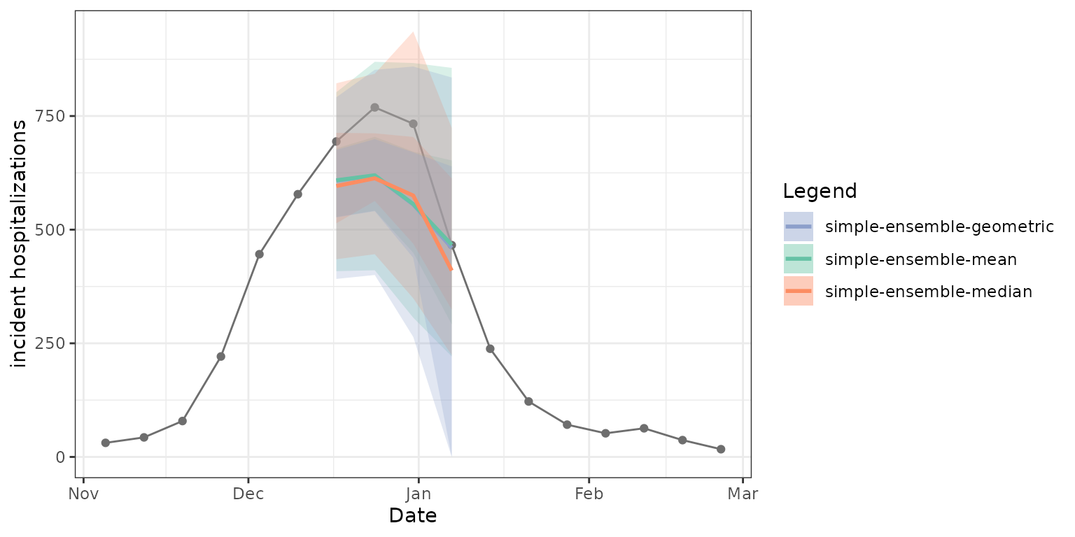
)As expected, the mean, median, and geometric mean each give us slightly different resulting ensembles. The median point estimates, 50% prediction intervals, and 90% prediction intervals in the figure below demonstrate this. Note that the geometric mean ensemble and simple mean ensemble generate similar estimates in this case of predicting weekly incident influenza hospitalizations in Massachusetts.
Weighting model contributions
We can weight the contributions of each model in the ensemble using
the weights argument of simple_ensemble().
This argument takes a data.frame that should include a
model_id column containing each unique model ID and a
weight column. In the following example, we include the
baseline model in the ensemble, but give it less weight than the other
forecasts.
model_weights <- data.frame(
  model_id = c("MOBS-GLEAM_FLUH", "PSI-DICE", "Flusight-baseline"),
  weight = c(0.4, 0.4, 0.2)
)
weighted_mean_ens <- hubExamples::forecast_outputs |>
  dplyr::filter(output_type != "sample") |>
  hubEnsembles::simple_ensemble(
    weights = model_weights,
    model_id = "simple-ensemble-weighted-mean"
  )
head(weighted_mean_ens, 10)
#> # A tibble: 10 × 9
#>    model_id                      location reference_date horizon target_end_date target           output_type output_type_id  value
#>    <chr>                         <chr>    <date>           <int> <date>          <chr>            <chr>       <chr>           <dbl>
#>  1 simple-ensemble-weighted-mean 25       2022-11-19           0 2022-11-19      wk flu hosp rate cdf         0.25           0.0129
#>  2 simple-ensemble-weighted-mean 25       2022-11-19           0 2022-11-19      wk flu hosp rate cdf         0.5            0.115
#>  3 simple-ensemble-weighted-mean 25       2022-11-19           0 2022-11-19      wk flu hosp rate cdf         0.75           0.546
#>  4 simple-ensemble-weighted-mean 25       2022-11-19           0 2022-11-19      wk flu hosp rate cdf         1              0.805
#>  5 simple-ensemble-weighted-mean 25       2022-11-19           0 2022-11-19      wk flu hosp rate cdf         1.25           0.910
#>  6 simple-ensemble-weighted-mean 25       2022-11-19           0 2022-11-19      wk flu hosp rate cdf         1.5            0.964
#>  7 simple-ensemble-weighted-mean 25       2022-11-19           0 2022-11-19      wk flu hosp rate cdf         1.75           0.989
#>  8 simple-ensemble-weighted-mean 25       2022-11-19           0 2022-11-19      wk flu hosp rate cdf         10             1
#>  9 simple-ensemble-weighted-mean 25       2022-11-19           0 2022-11-19      wk flu hosp rate cdf         10.25          1
#> 10 simple-ensemble-weighted-mean 25       2022-11-19           0 2022-11-19      wk flu hosp rate cdf         10.5           1
Creating ensembles with linear_pool
The linear_pool() function implements the linear opinion
pool (LOP, also known as a distributional mixture) method when
ensembling predictions. This function can be used to combine predictions
with output types mean, quantile, CDF, and PMF. Unlike
simple_ensemble(), this function handles its computation
differently based on the output type. For the CDF, PMF, and mean output
types, the linear pool method is equivalent to calling
simple_ensemble() with a mean aggregation function, since
simple_ensemble() produces a linear pool prediction (an
average of individual model cumulative or bin probabilities).
For the quantile output type, the linear_pool() function
first must approximate a full probability distribution using the
value-quantile level pairs from each component model. As a default, this
is done with functions in the distfromq package, which
defaults to fitting a monotonic cubic spline for the interior and a
Gaussian normal distribution for the tails. Quasi-random samples are
drawn from each distributional estimate, which are then collected and
used to extract the desired quantiles from the final ensemble
distribution.
Using the default options for linear_pool(), we can
generate an equally-weighted linear pool for each of the output types in
our example hub (except for the median and sample output types, which
must be excluded). The resulting distribution for the linear pool of
quantiles is estimated using a default of n_samples = 1e4
quasi-random samples drawn from the distribution of each component
model.
linear_pool_norm <- hubExamples::forecast_outputs |>
dplyr::filter(!output_type %in% c("median", "sample")) |>
hubEnsembles::linear_pool(model_id = "linear-pool-normal")
head(linear_pool_norm, 10)
#> # A tibble: 10 × 9
#> model_id location reference_date horizon target_end_date target output_type output_type_id value
#> <chr> <chr> <date> <int> <date> <chr> <chr> <chr> <dbl>
#> 1 linear-pool-normal 25 2022-11-19 0 2022-11-19 wk flu hosp rate cdf 0.25 0.0176
#> 2 linear-pool-normal 25 2022-11-19 0 2022-11-19 wk flu hosp rate cdf 0.5 0.118
#> 3 linear-pool-normal 25 2022-11-19 0 2022-11-19 wk flu hosp rate cdf 0.75 0.550
#> 4 linear-pool-normal 25 2022-11-19 0 2022-11-19 wk flu hosp rate cdf 1 0.819
#> 5 linear-pool-normal 25 2022-11-19 0 2022-11-19 wk flu hosp rate cdf 1.25 0.919
#> 6 linear-pool-normal 25 2022-11-19 0 2022-11-19 wk flu hosp rate cdf 1.5 0.968
#> 7 linear-pool-normal 25 2022-11-19 0 2022-11-19 wk flu hosp rate cdf 1.75 0.990
#> 8 linear-pool-normal 25 2022-11-19 0 2022-11-19 wk flu hosp rate cdf 10 1
#> 9 linear-pool-normal 25 2022-11-19 0 2022-11-19 wk flu hosp rate cdf 10.25 1
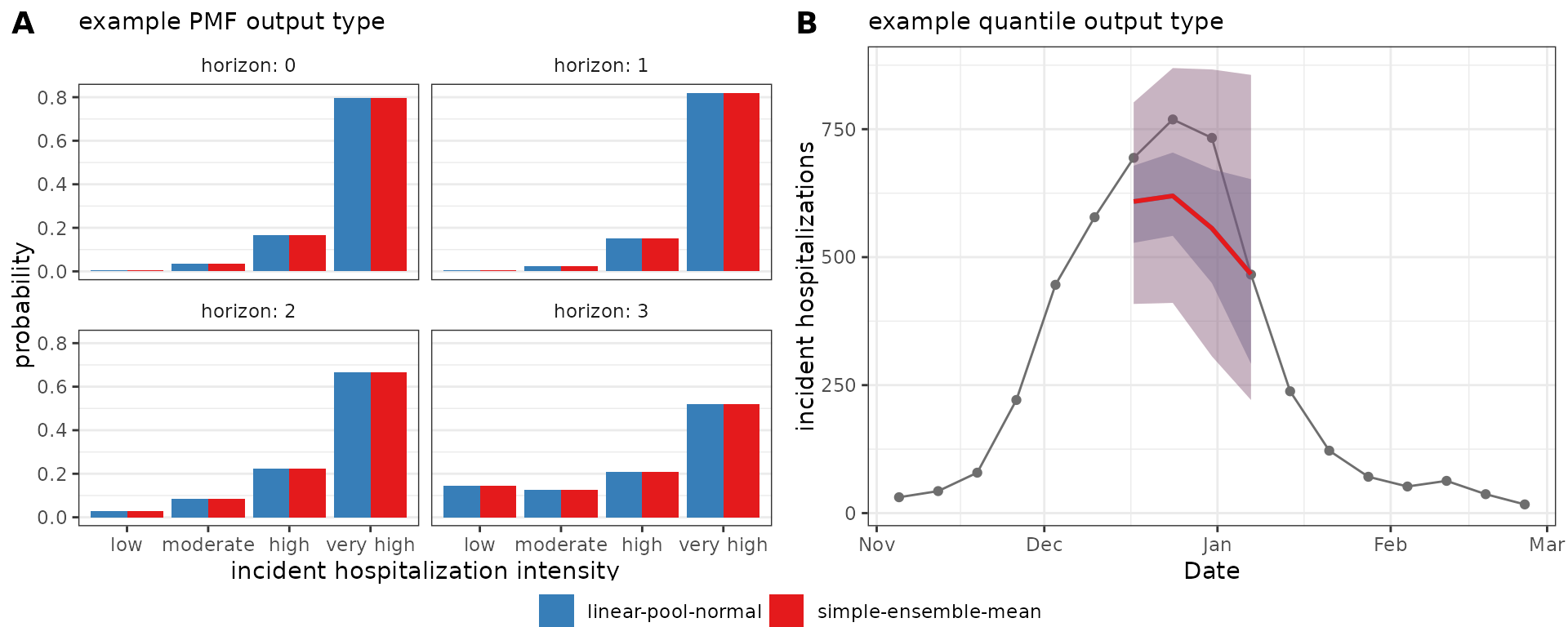
#> 10 linear-pool-normal 25 2022-11-19 0 2022-11-19 wk flu hosp rate cdf 10.5 1In the figure below, we compare ensemble results generated by
simple_ensemble() and linear_pool() for model
outputs of output types PMF and quantile. Panel A shows PMF type
predictions of Massachusetts incident influenza hospitalization
intensity while Panel B shows quantile type predictions of Massachusetts
weekly incident influenza hospitalizations. As expected, the results
from the two functions are equivalent for the PMF output type: for this
output type, the simple_ensemble() method averages the
predicted probability of each category across the component models,
which is the definition of the linear pool ensemble method. This is not
the case for the quantile output type, because the
simple_ensemble() is computing a quantile average.
Like with simple_ensemble(), we can change the default
aggregation settings. For example, weights that determine a model’s
contribution to the resulting ensemble may be provided.
model_weights <- data.frame(
  model_id = c("MOBS-GLEAM_FLUH", "PSI-DICE", "Flusight-baseline"),
  weight = c(0.4, 0.4, 0.2)
)
weighted_linear_pool_norm <- hubExamples::forecast_outputs |>
  dplyr::filter(!output_type %in% c("median", "sample")) |>
  hubEnsembles::linear_pool(
    weights = model_weights,
    model_id = "linear-pool-weighted"
  )
head(weighted_linear_pool_norm, 10)
#> # A tibble: 10 × 9
#>    model_id             location reference_date horizon target_end_date target           output_type output_type_id  value
#>    <chr>                <chr>    <date>           <int> <date>          <chr>            <chr>       <chr>           <dbl>
#>  1 linear-pool-weighted 25       2022-11-19           0 2022-11-19      wk flu hosp rate cdf         0.25           0.0129
#>  2 linear-pool-weighted 25       2022-11-19           0 2022-11-19      wk flu hosp rate cdf         0.5            0.115
#>  3 linear-pool-weighted 25       2022-11-19           0 2022-11-19      wk flu hosp rate cdf         0.75           0.546
#>  4 linear-pool-weighted 25       2022-11-19           0 2022-11-19      wk flu hosp rate cdf         1              0.805
#>  5 linear-pool-weighted 25       2022-11-19           0 2022-11-19      wk flu hosp rate cdf         1.25           0.910
#>  6 linear-pool-weighted 25       2022-11-19           0 2022-11-19      wk flu hosp rate cdf         1.5            0.964
#>  7 linear-pool-weighted 25       2022-11-19           0 2022-11-19      wk flu hosp rate cdf         1.75           0.989
#>  8 linear-pool-weighted 25       2022-11-19           0 2022-11-19      wk flu hosp rate cdf         10             1
#>  9 linear-pool-weighted 25       2022-11-19           0 2022-11-19      wk flu hosp rate cdf         10.25          1
#> 10 linear-pool-weighted 25       2022-11-19           0 2022-11-19      wk flu hosp rate cdf         10.5           1
We can also change the distribution that distfromq uses
to estimate the component models’ distributional tails to either log
normal or cauchy using the tail_dist argument. (See
documentation in the distfromq package for more details and
function options.) Note, though, that the choice of tail distribution
usually does not have a large impact on the resulting ensemble
distribution, except in its outer edges.
linear_pool_lnorm <- hubExamples::forecast_outputs |>
  dplyr::filter(!output_type %in% c("median", "sample")) |>
  hubEnsembles::linear_pool(
    model_id = "linear-pool-lognormal",
    tail_dist = "lnorm"
  )
linear_pool_cauchy <- hubExamples::forecast_outputs |>
  dplyr::filter(!output_type %in% c("median", "sample")) |>
  hubEnsembles::linear_pool(
    model_id = "linear-pool-cauchy",
    tail_dist = "cauchy"
  )